Saturday, November 23, 2013

Principle of Effective Demand: Aggregate Demand and Aggregate Supply Introduction

Principle of Effective Demand: Aggregate Demand and Aggregate Supply
Introduction
            The logical starting point of Keynes’s theory of employment is the principle of effective demand. In a entrepreneurial economy, the level of employment is based on effective demand. Thus employment results from a deficiency of effective demand and the level of employment can be raised by increasing the level of effective demand.
Aggregate Demand Price
       “The aggregate demand price for the output of any given amount of employment is the total sum of money or proceeds which is expected from the sale of the output produced when that amount of labor is employed.” Thus the aggregate demand price is the amount of money which the entrepreneurs expect to get by selling the output produced by the number of men employed. In other words it refers to the expected revenue from the sale of output produced at a particular level of employment. Different aggregate demand prices relate to different levels of employment in the economy.
       A statement showing the various aggregate demand prices at different levels of employment is called the aggregate demand price schedule or aggregate demand function. “The aggregate demand function.” according to Keynes, “relates any given level of employment to the expected proceeds from that level of employment.”
       The below tablet represents the aggregate demand schedule where it reveals that, with the increase in the level of employment proceeds, expected rise and at lower levels of employment decline. When 900 thousand people are provided employment the aggregate demand price is $560 million and when 250 thousand people are provided jobs, it is $480 million.
   
According to Keynes the aggregate demand function is an increasing function of the level of employment and is expressed as D = F (N), where D is the proceeds which entrepreneurs expect from the employment of N men.
Level of Employment
In 100 thousands
Aggregate Demand Price (D)
In Million $
4
460
5
480
6
500
7
520
8
540
9
560
10
580
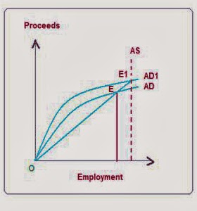
       The aggregate demand curve can be drawn on the basis of the above schedule. It inclines upward from the left to right for the reason that the level of employment increases aggregate demand price also rises, shown as AD curve in the upcoming diagram 1.


Aggregate Supply Price
            When an entrepreneur gives employment to a definite amount of labor, it requires certain quantities of co-operant factors like land, capital, raw materials etc. which will be paid remuneration along with labor. Thus each level of employment involves certain money costs of production including normal profits which the entrepreneur must cover. “At any given level of employment of labor aggregate supply price is the total amount of money which all the entrepreneurs in the economy, taken together must expect to receive from the sale of the output produced by that given number of men, if it is to be just worth employing them.”
            In brief, the aggregate supply price refers to the proceeds necessary from the sale of output at a particular level of employment. Thus each level of employment in the economy is related to a particular aggregate supply price and these are different aggregate supply prices for different levels of employment.
            A statement showing the various aggregate supply prices at different levels of employment is called aggregate supply price schedule or aggregate supply function. In the words of Prof. Dillard, “The aggregate supply function is a schedule of the minimum amounts of proceeds required to induce varying quantities of employment.” The below tablet reveals the aggregate supply schedule,

Level of Employment (N)
in 100 Thousands
Aggregate Supply Prize (Z)
In Million $
4
430
5
460
6
490
7
520
8
550
9
580
10
610


            The above table reveals that the aggregate supply prices rise with the hike in the level of employment. If entrepreneurs are to provide employment to 400 thousand workers, they must receive $430 millions from the sale of output produced by them. It is only when they expect to receive minimum amounts of proceeds ($460 millions, $490 million and $520 million) that they will provide employment to more workers (5, 6 and 7 hundred thousand dollars respectively).
            But when the economy reaches the level of full employment (at 800 thousand workers, the aggregate supply price ($550 million, $580 million and $610 millions) continues to increase but there is no further is an increasing function of the level of employment and is expressed as Z = ɸ N, Z is the aggregate supply price of the output level from employing N men.
            The aggregate supply curve can be drawn on the basis of the schedule. It inclines upward from left ro right for the reason that the necessary expected proceeds hikes; the level of employment also rises. But when the economy reaches the level of full employment, the aggregate supply curve becomes vertical. Even with the hike in the aggregate supply price, it is not possible to provide more employment as the economy has attained the level of full employment.


Reflationary policies and Deflationary policies

Reflationary policies and Deflationary policies


Keynesians - Policies                                  

The other sections about Keynesians show that they believe that the economy can settle at any equilibrium. This means that they recommend that the government gets actively involved in the economy to manage the level of demand. You will then be stunned to learn that these policies are known as demand-management policies.
Demand management means adjusting the level of demand to try to ensure that the economy arrives at full employment equilibrium. If there is a shortfall in demand, such as in a recession (a deflationary gap) then the government will need to reflate the economy. If there is an excess of demand, such as in a boom, then the government will need to deflate the economy.


Reflationary policies

Reflationary policies to boost the level of economic activity might include:

    * Increasing the level of government expenditure
    * Cutting taxation (either direct or indirect) to encourage spending
    * Cutting interest rates to encourage saving
    * Allowing some money supply growth

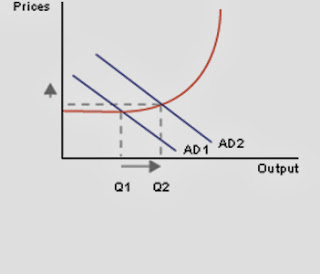
The first two policies would be considered expansionary fiscal policies, while the second two are expansionary monetary policies. The impact of them should be to reduce aggregate demand and therefore the level of output. The diagram below shows this:


[Reflationary policies] 


The reflationary policies have boosted the level of output from Q1 to Q2. The impact on the price level has been small, though if demand increased any more it may well be inflationary.

Deflationary policies

Deflationary policies to dampen down the level of economic activity might include:
    * Reducing the level of government expenditure
    * Increasing taxation (either direct or indirect) to discourage spending
    * Increasing interest rates to discourage saving
    * Reducing money supply growth

The first two policies would be considered contractionary fiscal policies, while the second two are contractionary monetary policies. The impact of them should be to reduce aggregate demand and therefore the level of output. The diagram below shows this:


[Deflationary policies] 


The initial level of aggregate demand was inflationary - prices were increasing rapidly.  However, the deflationary policies have reduced demand to AD2 and thus reduced the level of inflation.


Tax

Tax:
In honor of the filing date for taxes here in the US (today), I thought we could take a look at all the different kinds of taxes that exist. Last year, I did a whole tax week that looks at some of these in greater detail. I encourage you to explore those if you want to know more about some of these taxes, but today’s post will be much shorter. This list is by no means absolute, there are hundreds of different kinds of taxes, but these are the primary sources of income for most governments, local and national.
Sales Tax: In the US, we most often see this tax as a method for states to raise revenue for themselves. Customers make purchases at the retail level (not wholesale) and pay a tax that is a percentage of the sales price. States vary the rates they charge, and the rate also varies based on the product. For example a t-shirt has one tax, food has another, and gas has still another. Some states do not have a sales tax (such as Delaware) while others may charge more than 8% on a transaction. Retailers don’t like sales taxes because they have to collect that tax from the customer. They’ll claim it deters certain sales, but I find that unlikely unless someone lives near a state border. Speaking of which, states love the sales tax since they can get revenue from people outside the state. Places where tourism is big obviously benefit quite a bit. It’s arguable that the sales tax is the fairest of all taxes. It is a tax on consumption. If you want to save on taxes, don’t buy stuff (or buy less). Those that make more money tend to consume more, so they’ll pay more taxes. The catch is near the poverty line, where almost all purchases are just for basic living.
Capital Gains Tax: This is a tax on the profit made from the sale of an asset. It’s most commonly cited when it comes to profits made from selling stocks. If you buy a share of Stock A at $10 and then sell it for $15 you have a $5 capital gain. You must pay taxes on this gain. Currently, the United States has a favorable tax treatment of capital gains thanks to the Bush tax cuts, however those are likely to be allowed to expire. States will also take a chunk of the capital gains. The great thing about this tax is it only taxes people with enough excess income to actually invest. In other words, it’s a tax the poor don’t have to think about. The problem with the capital gains tax is during times of high inflation the value of an asset may increase simply due to inflation. Selling it would result in a tax on nominal, but not real, profits. This was part of the reasoning behind the Bush cut.
Income Tax: This is the big fish. Most states and the federal government rely heavily on income taxes. It taxes the financial income of individuals and companies. Most systems tax income in different brackets. So a person making $30,000 a year will pay less as a % of their income than someone making $60,000 a year. This system provides governments with a relatively stable income, simply because our earnings tend to be predictable. People are taxed on gross income, while companies generally are taxed on net income (profits). The downside for individuals is they tend to overpay their taxes every year and receive a refund. Though this is often celebrated, the net effect is giving the government a free short-term loan. That money could have been used by the individual to retire debt or invest. In the US, the income tax system is regularly criticized for being too complicated.
Property Tax: Like all taxes, this one is self-explanatory. It’s a tax based on the value of an asset. The most common reference is to a tax on your home, but it also includes your car and anything else the government wants to tax. The government is generally responsible for establishing the tax value of an asset, and they have a tendency to be conservative, but not always. Interestingly, the focus is on private assets in public view, such as your home, car, or boat. But if you loan a piece of art to a museum it can now be subject to the property tax. Like the capital gains tax, this tax tends to get revenue from those that make enough to obtain assets worth taxing.
Value Added Tax: This tax is familiar to our friends in Europe. It’s more complicated than a sales tax or income tax, but potentially more appropriate. Imagine a sales tax at every point in the supply chain. Generally, each stop in the chain of a product being converted from raw materials to something worth buying, has value added to it. So in the gas industry you might have 3 stops. The first group pumps oil and sells it to the refiner – tax. The refiner converts the oil to gasoline and sells it to gas station – tax. You pump the gas and pay the station – tax. Like any system it has its holes that allow people to commit fraud, but nothing is perfect. This system is also considered the most fair, since everyone gets taxed based on the contribution they make to the economy.
Regressive Tax: A tax that is less strenuous on the rich as it is on the poor. Sales taxes like that used in the US and the VAT in Europe are regressive taxes. The US income tax is the opposite in that it is progressive; the more you make, the more your tax burden is. Tariff: A tax designed to discourage a behavior. It’s most often applied on imports to protect domestic industries. Russia might impose a wheat tariff so that it’s more expensive for Russians to import wheat than just buy the wheat grown in the country. Tariffs are very disruptive on free markets and pricing.

Fair Tax: A tax system that is a universal sales tax. It was proposed as a solution to the complicated tax code the US currently has. It is a regressive tax, however breaks for the poor could be made to make it work.

Unemployment rate

Measuring the Unemployment rate
The unemployment rate is measured by dividing the number of unemployed workers by the total number of workers in the labor force. To be a member of the labor force, one has to be able and willing to work. Those who don't meet these criteria are excluded from the labor force. Those excluded aren't being counted as members of the labor force are, children below 16 years of age, full-time students and retirees who are neither working nor looking for a job even on a part-time basis, people on long-term care or in prison, home-makers, and all other unemployed people who are not actively looking for a job at least for a month. In the US, Japan, and Sweden, data on the number of unemployed workers is collected through telephone surveys to households whereas in other European countries the data is collected from unemployment claims register. The OECD office estimates that of the total number of unemployed people in Europe, only 80% register to claim unemployment compensation benefits. This suggests that the European method of reporting the unemployment rate underestimates the true rate of unemployment. In general, the unemployment rate in European countries is higher than in the US due to generous unemployment benefits extended to unemployed workers of European countries.
Frictional
This is the transitional or temporary unemployment that occurs when unemployed workers take time to search for a new job after losing or quitting their old job or after entering or re-entering the labor force following illness, schooling, etc. In a free society where individuals decide which jobs to accept or reject, frictional unemployment is unavoidable. Providing unemployed workers with information on available vacancies, can help to reduce the duration of frictional unemployment.
Structural
This type of unemployment is associated with relocation of firms or the fundamental changes in the structure of an economy. It results when the geographic location of a job seekers is different from the location of employers. For example, unemployment in the snow-belt areas of the north has been higher than the national average for many years following the relocation of the textile industry into the southern states where labor and energy costs are lower. Such a locational mismatch of vacancies and job seekers can be remedied either by relocation of workers into high growth regions or by creating enterprise zones to attract industries into economically depressed regions through tax incentives.
Structural unemployment can also result due to a mismatch between the skill requirement of vacancies & the available skill of job seekers. For example, due to declining demand for coal because of environmental concerns, the demand for coal miners has been shrinking over the years. In recent years, growing foreign competition has contributed to a high rate of unemployment in certain industries such as the textiles and steel industries. However, as jobs in the coal mining and heavy manufacturing industries are disappearing, new vacancies in the service sectors are being created. To the extent that the unemployed coal miners do not possess the required skills in the newly created vacancies of the service sector, they are likely to remain unemployed. Such an occupational mismatch of available skill of workers and skill requirements of vacancies can only be remedied through retraining of workers.
The main causes for structural unemployment: foreign trade, locational mismatch, tech (widens wage gap), minimum wage, and unions.
Seasonal
This is the type of unemployment that is associated with seasonal variations. For example, unemployment in the agricultural & construction sectors tends to increase in winter seasons. During the Christmas season, the unemployment rate tends to decrease throughout the economy. Since fluctuations of seasonal unemployment are fairly regular from one year to the next, the unemployment statistic makes an adjustment to account for this type of recurring seasonal variation. For example, if unemployment in the construction industry is one percent higher in January than the annual average, the seasonally adjusted unemployment rate for the month of January, is reported by subtracting one percentage point from the unadjusted unemployment rate.
Cyclical
Cyclical unemployment is caused by deficiency of aggregate demand or by unfavorable supply shocks. Cyclical unemployment is associated with recessions and can be reduced through expansionary macro economic policies (i.e. fiscal and monetary policies).
Natural
Natural unemployment is the sum total of frictional, seasonal and structural. It is the unemployment rate which can occur even when cyclical unemployment is zero. Reducing the natural rate of unemployment requires microeconomic policies that target specific unemployment area or a specific group of long-term unemployed workers.

The unemployment rate is calculated as: 

Unemployed/labor force x 100 (It is expressed as a percentage of the labor force.) 

The labor force is = employed + unemployed 

EconoMaldives: Pros and Cons of Direct Taxes

EconoMaldives: Pros and Cons of Direct Taxes

EconoMaldives: Pros and Cons of Indirect Taxes

EconoMaldives: Pros and Cons of Indirect Taxes

Friday, November 22, 2013

The Keynesian Model of Income Determination in a Three Sector Economy - Introduction of the Government Sector

The Keynesian Model of Income Determination in a Three Sector Economy - Introduction of the Government Sector
Introduction
            The action of government relating to its expenditures, transfers and taxes is called the fiscal policy. Here we focus on three fiscal policy models which are in increasing order of complexity, with the emphasis being on the government expenditure, taxation and the income level.
Determination of Equilibrium Income or Output In a Three Sector Economy
Though the government is involved in a variety of activates three of them are of greater relevance to us in the present context. Hence we will focus on these activities of the government, which are discussed below:
  1. Government Expenditure
This includes goods purchased by the central, state and the local government and also the payments made to the government employees.
  1. Transfers
These are those government payments which do not involve any direct services by the recipient for instance welfare payments, unemployment insurance and others.
  1. Taxes
These include taxes on property, income and goods. Taxes can be classified into two categories, direct taxes and indirect taxes. Direct taxes are levied directly and include personal income and corporate income tax. They are paid as a part of the price of the goods.
We simplify our analysis by making a few postulations, which are as follows.
  1. The government purchases factor services from the household sector and goods and services from the firms.

  1. Transfer payment includes subsidies to the firms and pensions to the household sector.

  1. The government levels only direct taxes on the household sector. We here introduce the notion of an income leakage and an injection. In a two sector model, a part of the current income stream leaked out as saving whereas injections in the form of investment were injected into the system.
In a three sector model taxes, like saving, are income leakages whereas government expenditures like investment are injections.
Let us see few illustrations relating to a three sector economy.
Illustration 21
In a two sector economy, the basic equations are as follows:
The Consumption function is C = 200 + 0.8Yd and investment is I = 300 millions. The equilibrium level of income is 2500 millions. Presume the government is added to this two sector model, which then becomes a three sector economy. The government expenditure is at 100 millions
  1. Determine the equilibrium level of income in the three sector economy
  2. What is the multiplier affect of the government expenditure? Is it of the same magnitude as the multiplier effect of a change in the autonomous investment?
  3. Presume that there is a balanced budget in that the entire government expenditure is financed from a lump sum tax. Find the new equilibrium level of income in the three sector economy.
Solution
The equilibrium condition in the three sector economy is given as
                                    Y         =          C + I + G
Thus,
                                    Y         =          200 + 0.8Y + 300 + 100
                                    Y         =          600 + 0.8Y
                        Y – 0.8Y         =          600
                                    0.2Y    =          600
                                    Y         =          600 / 0.2
The equilibrium level of income in the three sector economy is 3,000 millions, which is an increase by 500 millions over the two sector economy.
Government Expenditure Multiplier
                                    GM       =          Δ Y      =             1    
                                                            Δ G                    1 – b
                                                =          1 / 1 – 0.80
                                                =          5
Investment Multiplier, m        =         Δ Y      =               1        
                                                      Δ I                     1 – b
Where b is the marginal propensity to consume,
Thus the magnitude of the multiplier effect is the same as that of a change in government expenditure.
                                    G         =          T          =          100 millions
Thus,
                                    C         =          200 + 0.8 (Y -100)
                                    C         =          200 – 80 + 0.8Y
                                    C         =          120 + 0.8Y
But,                             Y         =          C + I + G
                                    Y         =          120 + 0.8Y + 300 + 100
                        Y – 0.8Y         =          120 + 400
                                    0.2Y    =          520
                                   Y         =          520 / 0.2
The new equilibrium level of income in the three sector economy, when there exists a balanced budget is 2,600 millions.
Illustration 22
In an economy, the full employment output occurs at 2000 millions. The marginal propensity to consume is 0.8 and the equilibrium level of output is currently at 1600 millions. Suppose the government aspires to achieve the full employment output, find the change in
  1. The level of government expenditures
  2. Net lump sum tax
  3. The level of government expenditures and the net lump sum tax when the government aims at bringing the productivity the full employment while keeping the budget balanced
Solution
We have, GM   =
Δ Y      =            1       
Δ G                  1 - b
Where, Δ G     =          Change in government expenditure
            b          =          Marginal propensity to consume
            Δ Y      =          Change in income
            GM       =          Government expenditure multiplier
For instance,
            b          =          0.80
            Δ Y      =          2000 – 1600
            Δ Y      =          400
Thus,
                        400 / Δ G         =          1 / 1- 0.8
                                    Δ G      =          400 (0.2)
Thus, the level of government expenditures required to achieve the full employment output is 80 millions

We have, GF    =
                                    Δ Y      =          - b      
                                    Δ T                  1 – b
Where,
                                                            Δ T      =          Change in tax
                                                            b          =          marginal propensity to consume
                                                            Δ Y      =          Change in income
                                                            GF        =          Government tax multiplier
As the tax multiplier is negative, an increase in tax leads to a decrease in the equilibrium level of income.
For instance,
                                                b          =          0.80
                                                Δ Y      =          2000 – 1600 = 400
Thus,
                                                400      =          - 0.80   
                                                Δ T                  1 – 0.80
                                    -0.8 Δ T           =          400 (0.20)
The net lump sum tax is – 100 millions. There should be a decrease in lump sum tax by 100 millions
The next equation to solve is
                                                Δ Y      =              1               (-b Δ T + Δ )
                                                                          1 – b
But,                                         Δ G      =          Δ T
Thus we can write
                                                Δ Y      =              1               (-b Δ
+ Δ )
                                                                          1 – b
Or
                                    Δ Y (1-b)         =          Δ
(-b +1)
Or                                Δ Y (1-b)         =          Δ (1-b)
Or                               
                                                Δ Y      =          1 – b    =          1
                                                Δ G      =          1 – b
                                                Δ Y      =          Δ G      =          400
The required increase in the level of government expenditures and the net lump sum tax us 400 millions.